Accessing data from large online rasters with Cloud-Optimized-Geotiff, GDAL, and terra R package

Converting a raster into a cloud optimised geotiff

As explained in https://www.cogeo.org, converting a raster into a cloud-optimised-geotiff (COG) is really easy using gdal_translate:

gdal_translate in.tif out.tif -co TILED=YES -co COPY_SRC_OVERVIEWS=YES -co COMPRESS=DEFLATE

If you want to make such conversion within R, you could use gdalUtilities for example:

gdalUtilities::gdal_translate(src_dataset = in.tif, 
                              dst_dataset = out.tif,
                              co = matrix(c("TILED=YES", 
                                            "COPY_SRC_OVERVIEWS=YES", 
                                            "COMPRESS=DEFLATE"), 
                                          ncol = 1))

out.tif will now be a cloud-optimised-geotiff which you can host online in a webpage, file server, etc.

Accessing data from cloud optimised geotiffs with R

Accessing data from cloud optimised geotiffs is easy, fast, and efficient thanks to GDAL virtual file system.

Here we use terra R package, the successor of raster package, to extract daily climate data for Grazalema, a rainy town in southern Spain. First, let’s get the site coordinates:

site.coords <- data.frame(lon = -5.36878, lat = 36.75864)

The climate raster files (in cloud optimised geotiff format) are hosted online in an FTP server (note https works as well). There is one large (several GB) COG raster for every year, and each has one layer per day (i.e. 365 or 366 layers depending on leap years).

If we wanted to obtain climate data from these rasters using the traditional workflow, we would have to download many GB to our computer, even if interested in a single site. But using COG, we can extract data in a matter of seconds without having to download any entire raster.

For example, this is the url of the COG raster with daily precipitation data for 2010:

ftp://palantir.boku.ac.at/Public/ClimateData/v2_cogeo/AllDataRasters/prec/DownscaledPrcp2010_cogeo.tif

We are going to paste “/vsicurl/” before the url to enable GDAL virtual file system:

cog.url <- "/vsicurl/ftp://palantir.boku.ac.at/Public/ClimateData/v2_cogeo/AllDataRasters/prec/DownscaledPrcp2010_cogeo.tif"

Now let’s connect to the online raster using terra::rast

library(terra)

## terra version 1.2.13

ras <- rast(cog.url)

We can see that the connection works. These are the raster metadata:

ras

## class       : SpatRaster 
## dimensions  : 6030, 13920, 365  (nrow, ncol, nlyr)
## resolution  : 0.008333333, 0.008333333  (x, y)
## extent      : -40.5, 75.5, 25.25, 75.5  (xmin, xmax, ymin, ymax)
## coord. ref. : +proj=longlat +datum=WGS84 +no_defs 
## source      : DownscaledPrcp2010_cogeo.tif 
## names       : Dow_1, Dow_2, Dow_3, Dow_4, Dow_5, Dow_6, ...

Now let’s extract the precipitation at this site for each day of 2010. Using terra::extract it is as simple as:

cog.data <- terra::extract(ras, site.coords)

We have 365 values of precipitation, one per day:

cog.data[1:10]

##   ID Dow_1 Dow_2 Dow_3 Dow_4 Dow_5 Dow_6 Dow_7 Dow_8 Dow_9
## 1  1     0     0  1331  3311     0  1940  1671     0     0

cog.data[360:366]

##   Dow_359 Dow_360 Dow_361 Dow_362 Dow_363 Dow_364 Dow_365
## 1     142       0       0       0     222    1182     694

And extraction has been very fast!

system.time({
  ras <- rast(cog.url)
  terra::extract(ras, site.coords)
})

##    user  system elapsed 
##   0.378   0.085   0.462

We are obtaining data from a 4 GB online raster in less than a second, without having to download anything!

We could also obtain the data for a particular day, or subset of days (e.g. 6 January 2010):

ras <- rast(cog.url)
ras <- subset(ras, 6)  # get 6th layer only (6 January)
terra::extract(ras, site.coords)

##   ID Dow_6
## 1  1  1940

Or for several sites:

site.coords <- data.frame(lon = c(-5.6, -5.1), 
                          lat = c(36.5, 37.2))
site.coords

##    lon  lat
## 1 -5.6 36.5
## 2 -5.1 37.2

terra::extract(ras, site.coords)

##   ID Dow_6
## 1  1  2043
## 2  2  1705

Finally, we could also get a subset of the online raster (i.e. get a raster rather than a data frame).

For example, to get a raster of the precipitation around Grazalema town on 6 January 2010:

site.coords <- data.frame(lon = c(-5.6, -5.1), 
                          lat = c(36.6, 37.2))
site.area <- vect(site.coords)  # convert to terra vector object (SpatVector)
site.area

##  class       : SpatVector 
##  geometry    : points 
##  dimensions  : 2, 2  (geometries, attributes)
##  extent      : -5.6, -5.1, 36.6, 37.2  (xmin, xmax, ymin, ymax)
##  coord. ref. :  
##  names       :   lon   lat
##  type        : <num> <num>
##  values      :  -5.6  36.6
##                 -5.1  37.2

ras <- rast(cog.url)
ras <- subset(ras, 6)  # get 6th layer only

precip <- terra::crop(ras, site.area)
plot(precip)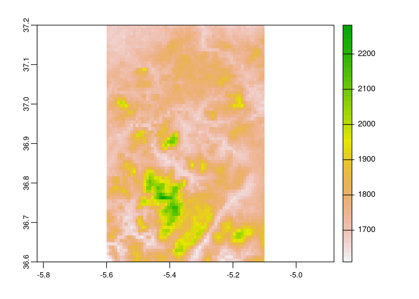

Conclusion

Cloud optimised geotiffs allow us to easily, quickly and efficiently distribute and access data from very large rasters hosted online.

We are using this approach in a forthcoming R package that aims to facilitate access to climate data. Stay tuned!