Using DHARMa to check Bayesian models fitted with brms
UPDATE 26 October 2022: There is now a DHARMa.helpers package that facilitates checking Bayesian brms models with DHARMa. Check it out!
The R package DHARMa is incredibly useful to check many different kinds of statistical models. It can be used with Bayesian models too, although it requires a few more lines of code.
Here I develop an example using DHARMa to check a Bayesian hierarchical generalised linear model fitted with the also fantastic brms package.
Example dataset
First, let’s simulate some count data with a hierarchical structure (random effect) and overdispersion:
library(DHARMa)testdata <- createData(sampleSize = 1000,
intercept = 0,
fixedEffects = 1,
numGroups = 20,
family = poisson(),
overdispersion = 0.5)
head(testdata)## ID observedResponse Environment1 group time x y
## 1 1 1 -0.68065204 1 1 0.2875775 0.2736227
## 2 2 0 -0.71096830 1 2 0.7883051 0.5938669
## 3 3 1 -0.70163922 1 3 0.4089769 0.1601848
## 4 4 1 0.02886852 1 4 0.8830174 0.8534302
## 5 5 0 -0.01434539 1 5 0.9404673 0.8477392
## 6 6 2 0.23268554 1 6 0.0455565 0.4778868We have simulated counts (observedResponse) in 20 sites as a function of an environmental variable (Environment1):
library(ggplot2)

ggplot(testdata) +
  geom_point(aes(Environment1, observedResponse)) +
facet_wrap(~group) 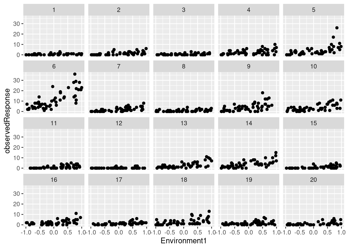
Fitting the model with brms
First, we try a non-hierarchical Poisson GLM of observed counts as a function of environment. For simplicity, using default priors here.
library(brms)model <- brm(observedResponse ~ Environment1,
data = testdata,
family = poisson(),
cores = 4)summary(model)## Family: poisson
## Links: mu = log
## Formula: observedResponse ~ Environment1
## Data: testdata (Number of observations: 1000)
## Draws: 4 chains, each with iter = 2000; warmup = 1000; thin = 1;
## total post-warmup draws = 4000
##
## Population-Level Effects:
## Estimate Est.Error l-95% CI u-95% CI Rhat Bulk_ESS Tail_ESS
## Intercept 0.69 0.03 0.64 0.74 1.00 1597 1974
## Environment1 1.05 0.04 0.97 1.14 1.00 1707 2047
##
## Draws were sampled using sampling(NUTS). For each parameter, Bulk_ESS
## and Tail_ESS are effective sample size measures, and Rhat is the potential
## scale reduction factor on split chains (at convergence, Rhat = 1).Model checking with DHARMa
To use DHARMa with brms (and other Bayesian packages), we must use the createDHARMa function, which takes the posterior simulations and the observed response to generate a DHARMa object, as simulateResiduals do with other supported model types.
model.check <- createDHARMa(
  simulatedResponse = t(posterior_predict(model)),
  observedResponse = testdata$observedResponse,
  fittedPredictedResponse = apply(t(posterior_epred(model)), 1, mean),
  integerResponse = TRUE)

plot(model.check)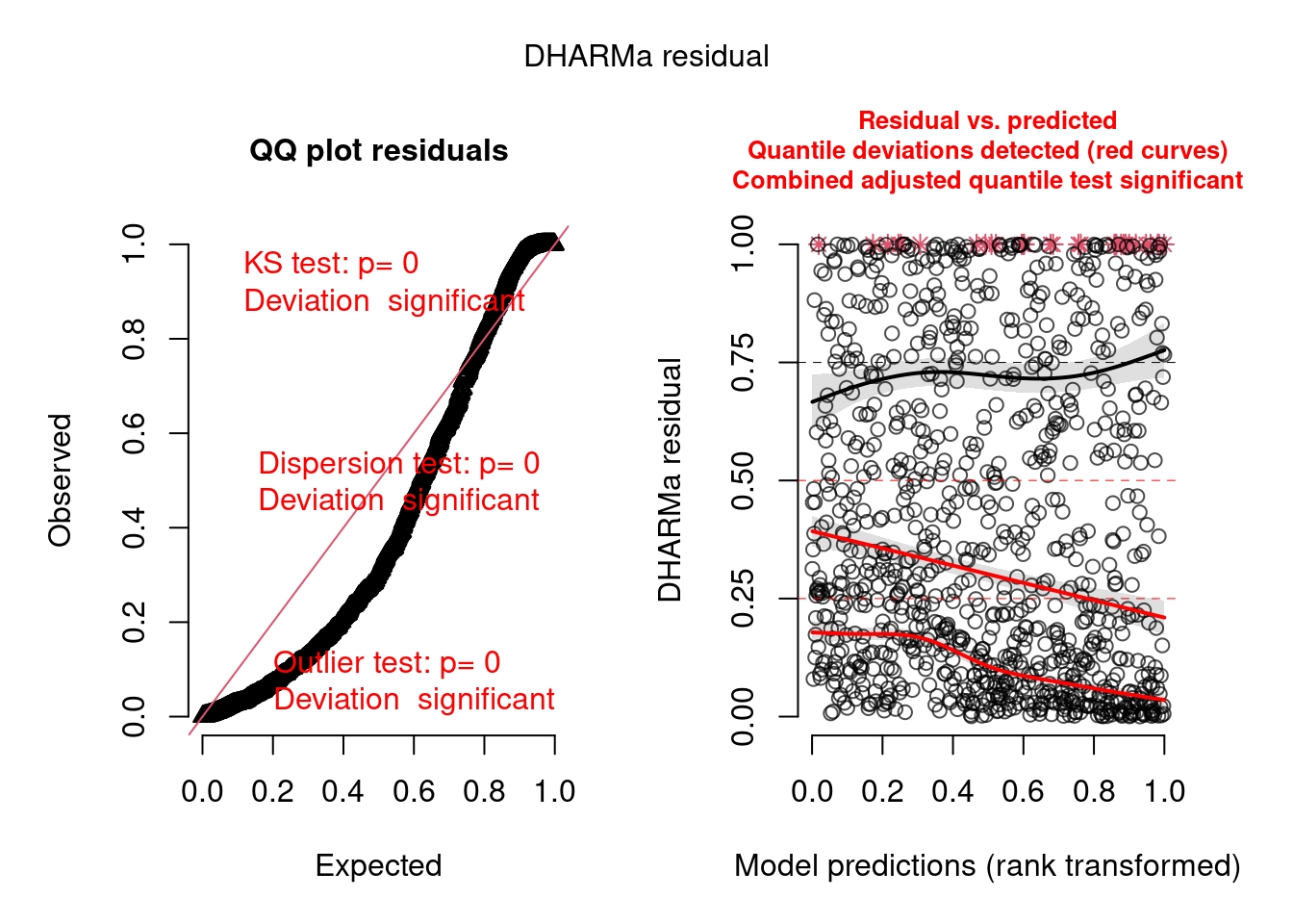
We can see there are problems with this model, which we will try to fix below. The posterior predictive check from bayesplot confirms the model is not adequate:
pp_check(model, nsamples = 100) + xlim(0, 20)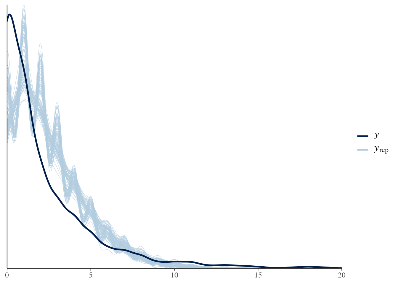
Automating DHARMa checks for brms models
To simplify the code, let’s write a function to automate the creation and examination of DHARMa objects from fitted brms models:
check_brms <- function(model,             # brms model
                       integer = FALSE,   # integer response? (TRUE/FALSE)
                       plot = TRUE,       # make plot?
                       ...                # further arguments for DHARMa::plotResiduals
) {

  mdata <- brms::standata(model)
  if (!"Y" %in% names(mdata))
    stop("Cannot extract the required information from this brms model")

  dharma.obj <- DHARMa::createDHARMa(
    simulatedResponse = t(brms::posterior_predict(model, ndraws = 1000)),
    observedResponse = mdata$Y,
    fittedPredictedResponse = apply(
      t(brms::posterior_epred(model, ndraws = 1000, re.form = NA)),
      1,
      mean),
    integerResponse = integer)

  if (isTRUE(plot)) {
    plot(dharma.obj, ...)
  }

  invisible(dharma.obj)

}
Note this function is used here for convenience and will not work with all brms models (e.g. models with more than one response).
Improving the model
Now, let’s try to fix the model. The DHARMa plot above shows that our model is not accounting for potential differences among groups (sites), and there is likely overdispersion (see DHARMa vignette for detailed explanations of how to interpret these plots).
Let’s start adding a varying intercept (random effect) to account for sites/groups:
model2 <- brm(observedResponse ~ Environment1 + (1 | group),
             data = testdata,
             family = poisson(),
             cores = 4,
iter = 4000)summary(model2)## Family: poisson
## Links: mu = log
## Formula: observedResponse ~ Environment1 + (1 | group)
## Data: testdata (Number of observations: 1000)
## Draws: 4 chains, each with iter = 4000; warmup = 2000; thin = 1;
## total post-warmup draws = 8000
##
## Group-Level Effects:
## ~group (Number of levels: 20)
## Estimate Est.Error l-95% CI u-95% CI Rhat Bulk_ESS Tail_ESS
## sd(Intercept) 0.95 0.18 0.68 1.37 1.00 877 1944
##
## Population-Level Effects:
## Estimate Est.Error l-95% CI u-95% CI Rhat Bulk_ESS Tail_ESS
## Intercept 0.33 0.21 -0.10 0.75 1.01 781 1209
## Environment1 1.05 0.04 0.97 1.12 1.00 3923 4460
##
## Draws were sampled using sampling(NUTS). For each parameter, Bulk_ESS
## and Tail_ESS are effective sample size measures, and Rhat is the potential
## scale reduction factor on split chains (at convergence, Rhat = 1).Check with DHARMa using the function we just created:
model2.check <- check_brms(model2, integer = TRUE)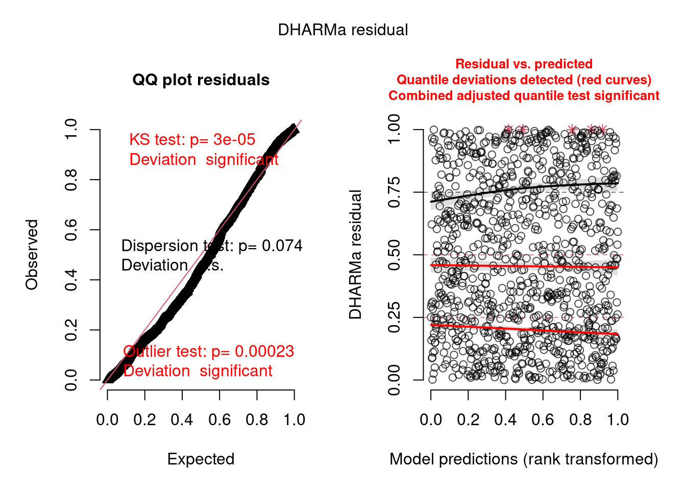
There are still problems, but the residuals show a better pattern now. They are now quite homogeneous among sites:
plot(model2.check, form = testdata$group)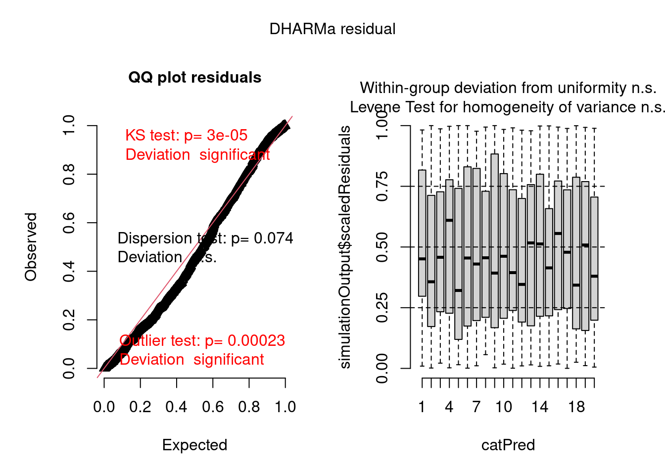
But there are still problems. One of them seems to be overdispersion:
testDispersion(model2.check)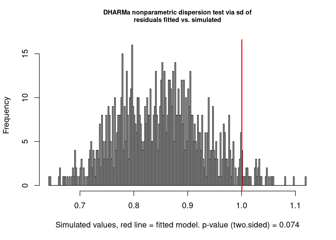
##
##  DHARMa nonparametric dispersion test via sd of residuals fitted vs.
##  simulated
##
## data:  simulationOutput
## dispersion = 1.1758, p-value = 0.074
## alternative hypothesis: two.sided
Improving the model further
Let’s add an observation-level random effect to try to account for overdispersion:
testdata$obs.id <- 1:nrow(testdata)

model3 <- brm(observedResponse ~ Environment1 + (1 | group) + (1 | obs.id),
             data = testdata,
             family = poisson(),
             cores = 4,
iter = 4000)summary(model3)## Family: poisson
## Links: mu = log
## Formula: observedResponse ~ Environment1 + (1 | group) + (1 | obs.id)
## Data: testdata (Number of observations: 1000)
## Draws: 4 chains, each with iter = 4000; warmup = 2000; thin = 1;
## total post-warmup draws = 8000
##
## Group-Level Effects:
## ~group (Number of levels: 20)
## Estimate Est.Error l-95% CI u-95% CI Rhat Bulk_ESS Tail_ESS
## sd(Intercept) 0.97 0.18 0.69 1.39 1.00 1552 2831
##
## ~obs.id (Number of levels: 1000)
## Estimate Est.Error l-95% CI u-95% CI Rhat Bulk_ESS Tail_ESS
## sd(Intercept) 0.45 0.04 0.38 0.52 1.00 3113 4371
##
## Population-Level Effects:
## Estimate Est.Error l-95% CI u-95% CI Rhat Bulk_ESS Tail_ESS
## Intercept 0.22 0.21 -0.20 0.63 1.00 854 1776
## Environment1 1.07 0.05 0.97 1.18 1.00 6430 6334
##
## Draws were sampled using sampling(NUTS). For each parameter, Bulk_ESS
## and Tail_ESS are effective sample size measures, and Rhat is the potential
## scale reduction factor on split chains (at convergence, Rhat = 1).Check:
model3.check <- check_brms(model3, integer = TRUE)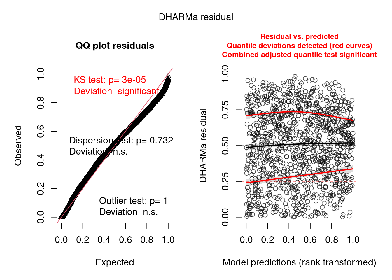
There are still some warnings, although the observation-level random effect seems to have corrected for overdispersion:
testDispersion(model3.check)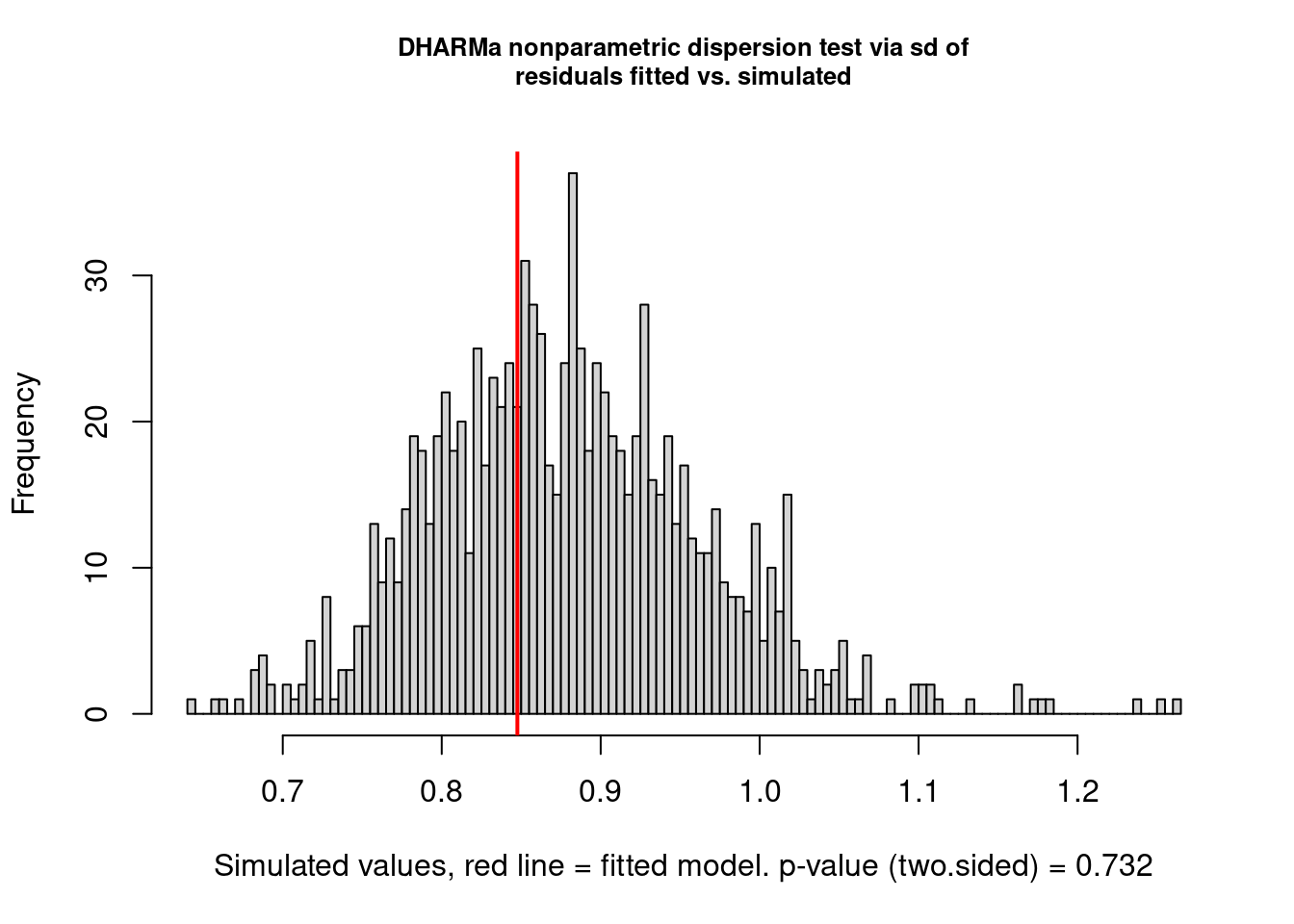
##
##  DHARMa nonparametric dispersion test via sd of residuals fitted vs.
##  simulated
##
## data:  simulationOutput
## dispersion = 0.96409, p-value = 0.732
## alternative hypothesis: two.sided
Improve the model even further
Let’s try using a negative binomial distribution rather than a Poisson:
model4 <- brm(observedResponse ~ Environment1 + (1 | group),
             data = testdata,
             family = negbinomial(),
             cores = 4,
             iter = 4000)

summary(model4)
## Family: negbinomial
## Links: mu = log; shape = identity
## Formula: observedResponse ~ Environment1 + (1 | group)
## Data: testdata (Number of observations: 1000)
## Draws: 4 chains, each with iter = 4000; warmup = 2000; thin = 1;
## total post-warmup draws = 8000
##
## Group-Level Effects:
## ~group (Number of levels: 20)
## Estimate Est.Error l-95% CI u-95% CI Rhat Bulk_ESS Tail_ESS
## sd(Intercept) 0.95 0.17 0.69 1.37 1.00 1098 1744
##
## Population-Level Effects:
## Estimate Est.Error l-95% CI u-95% CI Rhat Bulk_ESS Tail_ESS
## Intercept 0.31 0.22 -0.12 0.74 1.00 885 1613
## Environment1 1.07 0.05 0.97 1.17 1.00 4924 4697
##
## Family Specific Parameters:
## Estimate Est.Error l-95% CI u-95% CI Rhat Bulk_ESS Tail_ESS
## shape 4.81 0.75 3.57 6.45 1.00 5178 4762
##
## Draws were sampled using sampling(NUTS). For each parameter, Bulk_ESS
## and Tail_ESS are effective sample size measures, and Rhat is the potential
## scale reduction factor on split chains (at convergence, Rhat = 1).Check:
model4.check <- check_brms(model4, integer = TRUE)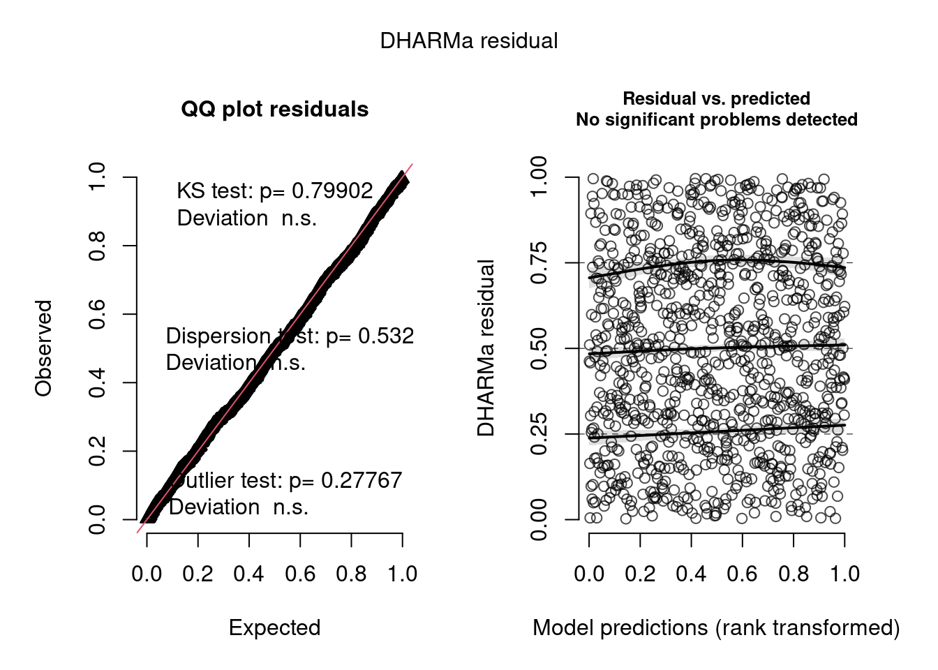
plot(model4.check, form = testdata$Environment1)
plot(model4.check, form = testdata$group)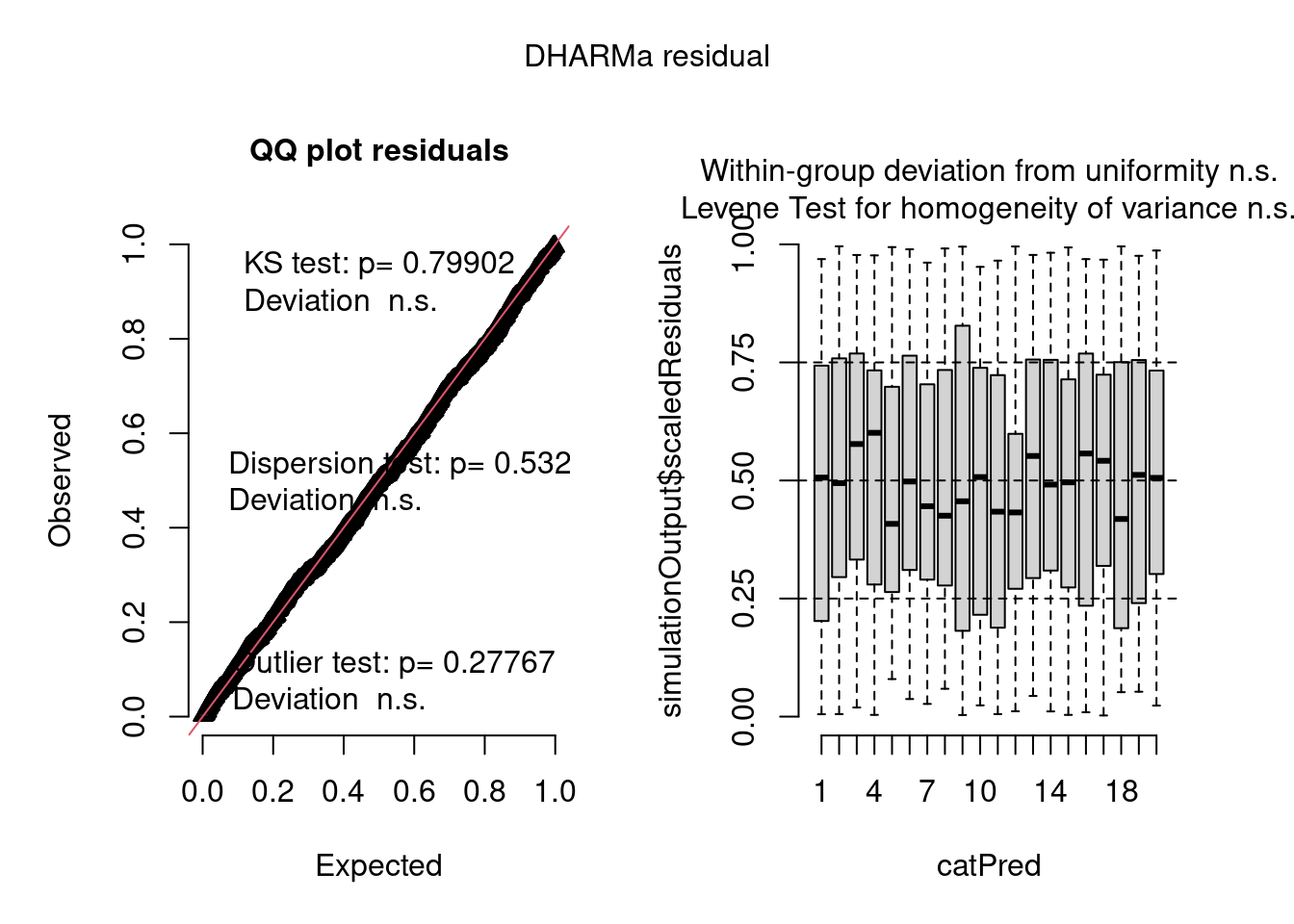
The negative binomial model looks better in this case.
Let’s check it with bayesplot too:
pp_check(model4, nsamples = 100) + xlim(0, 20)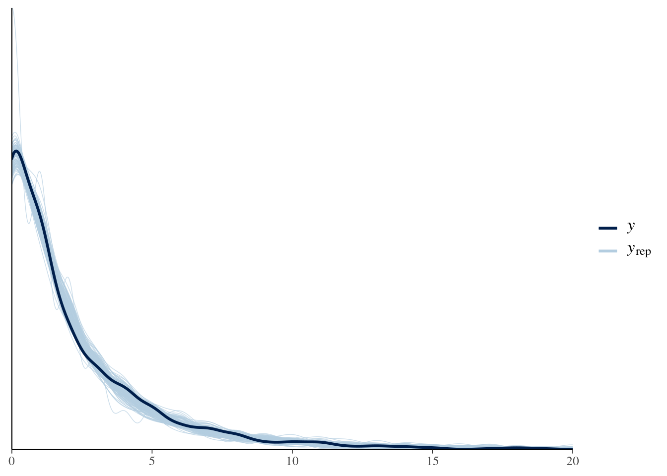
library(bayesplot)

ppc_rootogram(y = testdata$observedResponse,
              yrep = posterior_predict(model4, nsamples = 1000)) +
  xlim(0, 20)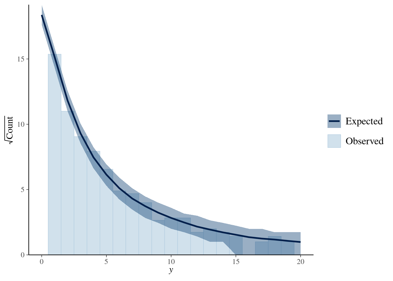
Conclusion
DHARMa can greatly facilitate thorough checking and improvement of Bayesian models, as those fitted with brms.
Prof. Florian Hartig kindly revised a draft of this post.