Bayesian inference of bipartite networks structure
Inferring the structure of bipartite (e.g. pollination, frugivory, or herbivory) networks from field (observational) data is a challenging task. Interaction data are hard to collect and require typically large sampling efforts, particularly to characterize infrequent interactions. Inferred network structure is highly sensitive to sampling design, effort, and completeness. Comparing networks from different studies without accounting for these sampling effects may lead to mistaken inferences.
Young et al. (2021) developed a Bayesian approach to infer the structure of bipartite networks from unreliable (observational) data. Here I present the BayesianWebs R package which facilitates modelling bipartite networks, such as mutualistic networks, using that Bayesian framework. In particular, BayesianWebs uses Bayesian modelling to infer the posterior probability of each pairwise interaction in bipartite networks, accounting for sampling completeness and the inherent stochasticity of field observation data.
Let’s see an example taken from my Ph.D. research on the interaction between frugivorous birds and laurel trees. These are the number of visits observed in the field:
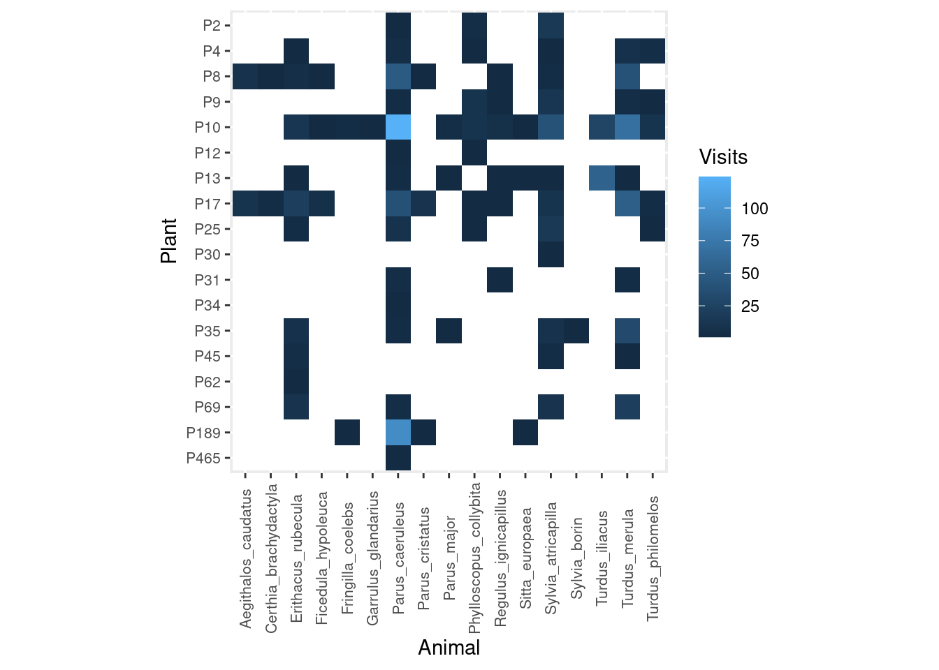
As you can see, I recorded many more bird visits to some plants (e.g. P10) than others (e.g. P12, P30, P465), and by a much wider diversity of animals.
Many network analyses would proceed by taking these observed counts for granted and deriving all network and node-level metrics without accounting for the inherent uncertainty in these data.
What if the sampling effort is not constant among plants? What if we are comparing networks with very different sampling efforts and thus different degrees of reliability?
In this case we have observed each plant for different number of hours. Obviously it is not the same to record 10 interactions in 1 hour than in 20 hours. We should account for that somehow. We could divide the observed counts by the sampling effort (hours observed) to get an “standardised” measure of interaction frequency “controlling for” varying sampling effort:
| Plant | Visits/h | hours |
|---|---|---|
| P10 | 0.79 | 23 |
| P35 | 0.52 | 6 |
| P69 | 0.42 | 6 |
| P189 | 0.38 | 15 |
| P17 | 0.36 | 25 |
| P8 | 0.36 | 18 |
| P13 | 0.30 | 13 |
| P25 | 0.23 | 7 |
| P2 | 0.11 | 11 |
| P9 | 0.10 | 19 |
| P45 | 0.07 | 7 |
| P4 | 0.06 | 18 |
| P62 | 0.06 | 1 |
| P31 | 0.05 | 9 |
| P12 | 0.04 | 4 |
| P30 | 0.03 | 2 |
| P34 | 0.03 | 2 |
| P465 | 0.02 | 3 |
We can see that some plants apparently receive many more visits per hour (0.52 visits/h in P35) than others (e.g. 0.1 visits/h in P9). And others apparently receive the same interaction frequency (e.g. 0.06 visits/h in P4 and P62) even though one has been monitored for 18 hours and the other for just 1 hour.
But our standardised measure of interaction frequency (Visits/h) has lost the information on the real sampling effort spent on each plant. For sure, the reliability (uncertainty) of the inferred interaction frequency per plant cannot be the same if we have observed a plant for 20 hours compared to just 1 hour.
Bayesian modelling of network structure
BayesianWebs allows us to easily infer the posterior probability of each pairwise interaction (and the predicted interaction frequency or number of visits) taking into account varying sampling efforts and the inherent uncertainty of interaction count data.
library("BayesianWebs")First, let’s prepare the data for modelling:
dt <- prepare_data(mat, sampl.eff = effort$hours)Now fit the model (here using 4 parallel chains):
set.seed(1)
options(mc.cores = 4)
fit <- fit_model(dt, refresh = 0)
## Running MCMC with 4 parallel chains...
##
## Chain 3 finished in 3.8 seconds.
## Chain 1 finished in 3.9 seconds.
## Chain 2 finished in 3.9 seconds.
## Chain 4 finished in 4.0 seconds.
##
## All 4 chains finished successfully.
## Mean chain execution time: 3.9 seconds.
## Total execution time: 4.2 seconds.This is the average posterior probability of each pairwise interaction:
post <- get_posterior(fit, data = dt)
plot_interaction_prob(post)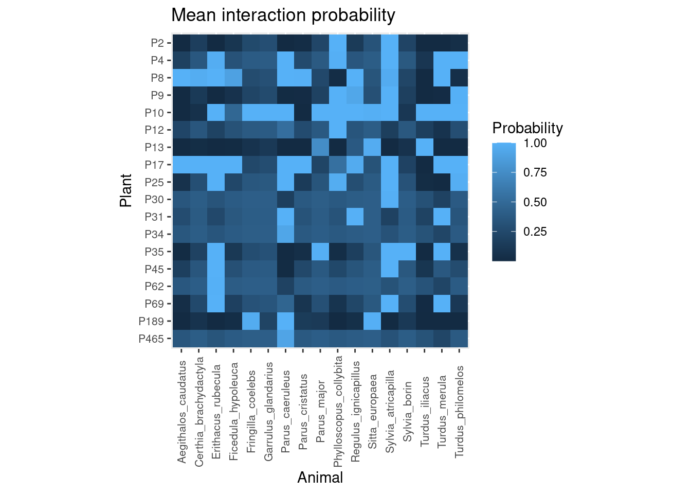
According to our model, plants like P10 have very high probability of interacting with most bird species, except Aegithalos caudatus, Certhya brachydactyla, Parus cristatus and Sylvia borin. In contrast, plants like P2 have low probabilities of interacting with most bird species except Phylloscopus collybita and Sylvia atricapilla.
Likewise, we can see that common birds like Erithacus rubecula or Sylvia atricapilla interact with most plants except P13 or P189. While other species, like Fringilla_coelebs show high probability of interacting with P189 and P10.
However, the most interesting output is that we have full posterior distributions behind those averages, so we can estimate the uncertainty regarding each pairwise interaction and propagate it downstream in further analyses. Here is the width of 95% Bayesian credible intervals for each interaction (the wider the interval, the more uncertainty):
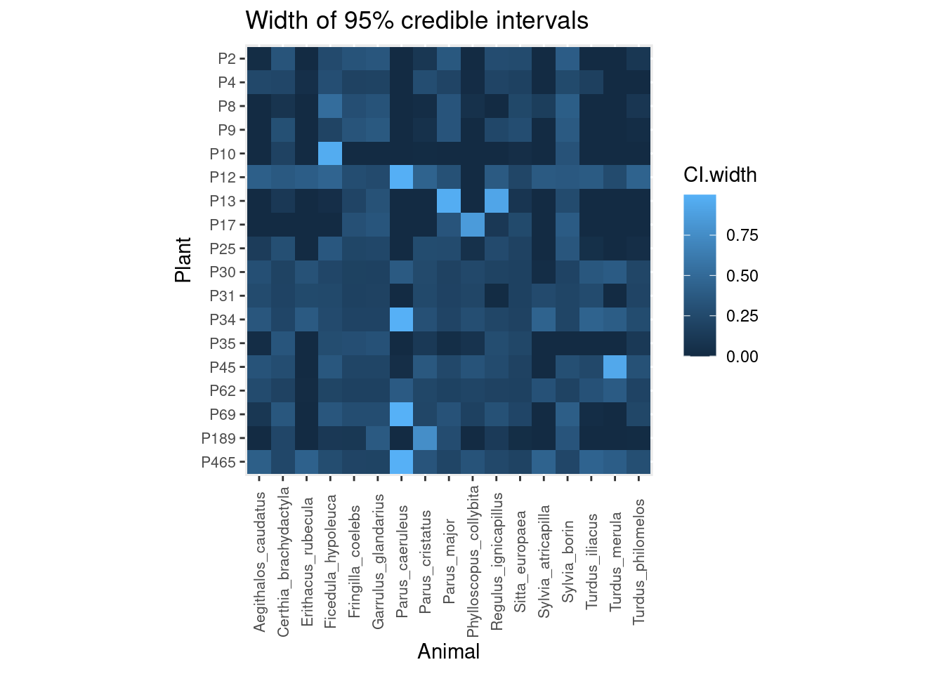
We can see that plants P10 and P17, which had the largest sampling effort (23 and 25 hours, respectively), show narrow credible intervals (i.e. low uncertainty) for most interactions, except for the interaction between P10 and Ficedula hypoleuca and P17 and Phylloscopus collybita. Likewise, interactions between Parus caeruleus and many plants are rather uncertain.
Finally, we can compare the observed interaction counts with those predicted by the model taking into account the interaction frequencies of each plant and animal:
pred.df <- predict_counts(fit, data = dt)
plot_counts_pred(pred.df, sort = FALSE)
plot_counts_obs(mat, sort = FALSE, zero.na = FALSE)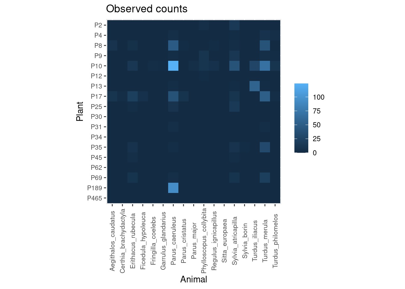
As you can see there is good agreement, even though the model is modifying slightly the expected number of visits for some interactions, based on interaction patterns of each plant and animal with the rest of the community. Some interactions are also much more certain than others:
plot_counts_pred_obs(pred.df, data = dt)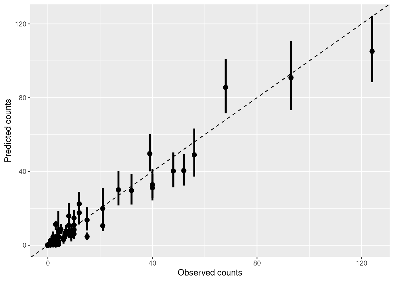
If you want to know more, please read Young et al. paper or visit the BayesianWebs website.